Pivot Tables in Excel are fine, right? They get the job done, but only until the moment you need to tweak the layout, add a new field, refresh the numbers after a new data dump arrives. Before you start scrambling through Excel’s UI, clicking through dozens of dialog boxes and dragging fields around hoping you don’t break something, know that there’s a better way.
Excel has hundreds of built-in formulas that let you do anything from simple arithmetic to, you guessed it, building Pivot Tables. And now that Excel can write its own formulas, there’s no reason why you shouldn’t be using its PIVOTBY function to rebuild the same summaries in minutes instead of hours.

Stop clicking—build Pivot Tables with formulas
A faster, more flexible way to create dynamic summaries

First introduced in Excel for Microsoft 365, PIVOTBY is a dynamic array function that produces essentially the same kind of cross-table summaries you’d get from a Pivot Table, except with zero manual refreshing and a lot more automation and flexibility. It shows resutls automatically in as many cells as required and automatically updates as the source data changes.
The formula itself isn’t complicated either. The syntax is simply:
PIVOTBY (row_fields, col_fields, values, function)
In the formula above, row_fields is the column you want running down the left side, col_fields is what runs across the top (generally a period of time), the values argument is the data you want to work with and function is how you want to calculate it — SUM, AVERAGE, COUNT — you name it, Excel can do it. There are other arguments to the formula available as well, but these are the four required arguments you need to provide for PIVOTBY to work.
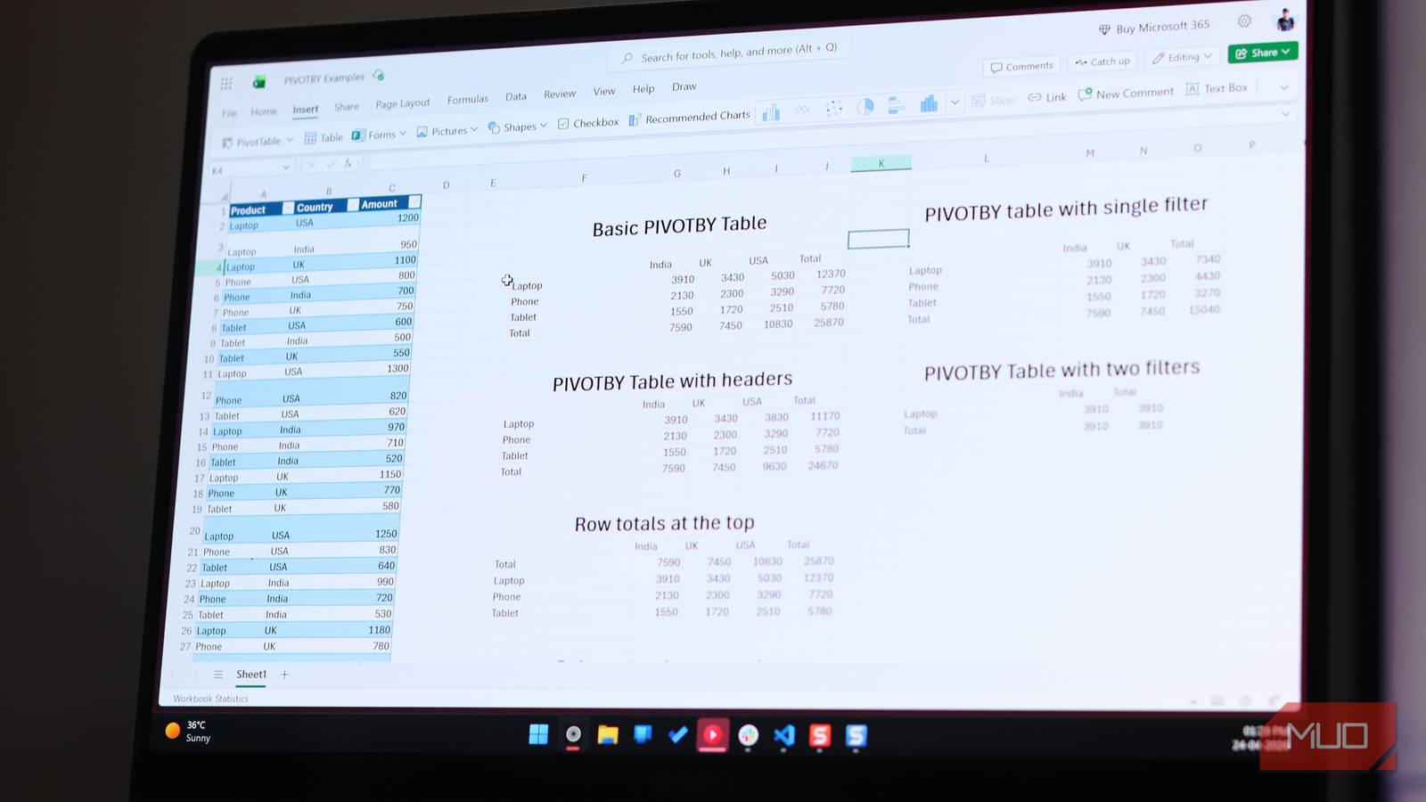
Let’s say you have a sales table with columns for Product, Country and Amount, and your current Pivot Table shows total sales by Product (in rows) and Country (in columns). To rebuild this view using the PIVOTBY formula, just use the following formula in an empty cell

=PIVOTBY(A2:A32, B2:B32, C2:C32, SUM)
As soon as you hit Enter, Excel does the rest. It’ll group, aggregate, and lay out the full table, and throw in grand totals by default.
- OS
-
Windows, macOS
- Supported Desktop Browsers
-
All via web app
- Developer(s)
-
Microsoft
- Free trial
-
One month
Changing layouts becomes effortless
Rearrange fields without rebuilding everything from scratch
As you can probably guess, recreating and fine-tuning PIVOTBY tables is also quite easy as compared to traditional Pivot Tables. For example, with a traditional Pivot Table, adding headers means going back into the field settings. With PIVOTBY, you can simply add a fifth parameter field_headers and choose to show the default headers or automatically generate them if they don’t exist in the source data. Want grand totals on the top instead of bottom? Set row_total_depth to -1. Want to remove column totals? Set col_total_depth to 0. Every Pivot Table tweak that you would have to fish through the Excel UI for is now a number in a formula.
Filtering data also becomes significantly easier with PIVOTBY. Complex filtering can be clunky in traditional Pivot Tables, but they can be written as regular expressions in PIVOTBY. For example, if you want to see only rows where Country isn’t the USA, add C2:C32″USA” at the end of your formula. Want to see a specific product from a specific country? Simply multiply two IF statements and the results will only include items that match both conditions. Regular Pivot Tables will have you adding fields into the Filters area or adding slicers all day long instead.
There are a few gotchas to know
Where this approach can trip you up

The one thing you need to keep in mind before using PIVOTBY is that it relies on Excel tables to pull off the kind of versatility it has. PIVOTBY doesn’t automatically expand when you add new rows to your raw data unless it’s formatted as an Excel table. If you’re still working with a plain data range, you can quickly convert it into a table by selecting the data and pressing Ctrl + T.
PIVOTBY also won’t automatically format the output for you, which Pivot Tables do. A standard Pivot Table will add banded rows, bold headers, and highlighted totals by default. PIVOTBY does no such thing, but you can use conditional formatting rules that apply automatically to the spill range. This means once you set it up, the formatting stays consistent as your data changes, expands, or shrinks. Excel also prompts its Quick Analysis tool when the output is generated, making formatting or charting easier.
Last but not least, there are still situations where the old-school Pivot Table is still better. If you need slicers connected to multiple visuals, if you’re working from a Power Pivot data model, or if your colleagues on older Excel versions need to interact with the file, Pivot Tables remain your only option.
PIVOTBY is limited to Excel for Microsoft 365, meaning compatibility is a big issue. If your existing Excel license doesn’t support PIVOTBY, Pivot Tables, once again, are the go-to choice. However, you don’t need to be a coder to use Python in Excel for data cleaning, so if that’s another use case for you, an upgrade to Microsoft 365 might make sense, courtesy of its built-in Python support. You can also use Copilot in Excel to make Pivot Tables easier.
There’s a smarter way to pull data
Cleaner inputs that make your analysis far more powerful
If you’re already comfortable with Pivot Tables, you’ve basically done the hard thinking PIVOTBY needs. You know what belongs in rows, what goes into columns, and which numbers matter. All you need to change is where that logic applies.

This Excel Trick Lets Me Write Formulas Like a Human
Smarter Excel formulas with the simplicity of everyday language.
The learning curve is quite small as well and a couple of references to the official documentation will get you up and running quickly. You really only need the first four arguments as mentioned above to get an output, and if you’ve been working with Pivot Tables, you already know what they are.
[ad_2]
Source link